AWS Machine Learning Blog
Monitoring Lake Mead drought using the new Amazon SageMaker geospatial capabilities
Earth’s changing climate poses an increased risk of drought due to global warming. Since 1880, the global temperature has increased 1.01 °C. Since 1993, sea levels have risen 102.5 millimeters. Since 2002, the land ice sheets in Antarctica have been losing mass at a rate of 151.0 billion metric tons per year. In 2022, the Earth’s atmosphere contains more than 400 parts per million of carbon dioxide, which is 50% more than it had in 1750. While these numbers might seem removed from our daily lives, the Earth has been warming at an unprecedented rate over the past 10,000 years [1].
In this post, we use the new geospatial capabilities in Amazon SageMaker to monitor drought caused by climate change in Lake Mead. Lake Mead is the largest reservoir in the US. It supplies water to 25 million people in the states of Nevada, Arizona, and California [2]. Research shows that the water levels in Lake Mead are at their lowest level since 1937 [3]. We use the geospatial capabilities in SageMaker to measure the changes in water levels in Lake Mead using satellite imagery.
Data access
The new geospatial capabilities in SageMaker offer easy access to geospatial data such as Sentinel-2 and Landsat 8. Built-in geospatial dataset access saves weeks of effort otherwise lost to collecting data from various data providers and vendors.
First, we will use an Amazon SageMaker Studio notebook with a SageMaker geospatial image by following steps outlined in Getting Started with Amazon SageMaker geospatial capabilities. We use a SageMaker Studio notebook with a SageMaker geospatial image for our analysis.
The notebook used in this post can be found in the amazon-sagemaker-examples GitHub repo. SageMaker geospatial makes the data query extremely easy. We will use the following code to specify the location and timeframe for satellite data.
In the following code snippet, we first define an AreaOfInterest (AOI) with a bounding box around the Lake Mead area. We use the TimeRangeFilter to select data from January 2021 to July 2022. However, the area we are studying may be obscured by clouds. To obtain mostly cloud-free imagery, we choose a subset of images by setting the upper bound for cloud coverage to 1%.
Model inference
After we identify the data, the next step is to extract water bodies from the satellite images. Typically, we would need to train a land cover segmentation model from scratch to identify different categories of physical materials on the earth surface’s such as water bodies, vegetation, snow, and so on. Training a model from scratch is time consuming and expensive. It involves data labeling, model training, and deployment. SageMaker geospatial capabilities provide a pre-trained land cover segmentation model. This land cover segmentation model can be run with a simple API call.
Rather than downloading the data to a local machine for inferences, SageMaker does all the heavy lifting for you. We simply specify the data configuration and model configuration in an Earth Observation Job (EOJ). SageMaker automatically downloads and preprocesses the satellite image data for the EOJ, making it ready for inference. Next, SageMaker automatically runs model inference for the EOJ. Depending on the workload (the number of images run through model inference), the EOJ can take several minutes to a few hours to finish. You can monitor the job status using the get_earth_observation_job function.
Visualize results
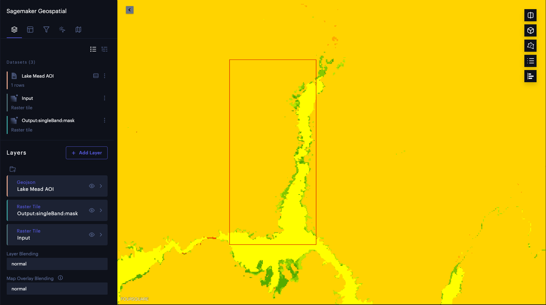
Now that we have run model inference, let’s visually inspect the results. We overlay the model inference results on input satellite images. We use Foursquare Studio tools that comes pre-integrated with SageMaker to visualize these results. First, we create a map instance using the SageMaker geospatial capabilities to visualize input images and model predictions:
When the interactive map is ready, we can render input images and model outputs as map layers without needing to download the data. Additionally, we can give each layer a label and select the data for a particular date using TimeRangeFilter:
We can verify that the area marked as water (bright yellow in the following map) accurately corresponds with the water body in Lake Mead by changing the opacity of the output layer.

Post analysis
Next, we use the export_earth_observation_job function to export the EOJ results to an Amazon Simple Storage Service (Amazon S3) bucket. We then run a subsequent analysis on the data in Amazon S3 to calculate the water surface area. The export function makes it convenient to share results across teams. SageMaker also simplifies dataset management. We can simply share the EOJ results using the job ARN, instead of crawling thousands of files in the S3 bucket. Each EOJ becomes an asset in the data catalog, as results can be grouped by the job ARN.
Next, we analyze changes in the water level in Lake Mead. We download the land cover masks to our local instance to calculate water surface area using open-source libraries. SageMaker saves the model outputs in Cloud Optimized GeoTiff (COG) format. In this example, we load these masks as NumPy arrays using the Tifffile package. The SageMaker Geospatial 1.0 kernel also includes other widely used libraries like GDAL and Rasterio.
Each pixel in the land cover mask has a value between 0-11. Each value corresponds to a particular class of land cover. Water’s class index is 6. We can use this class index to extract the water mask. First, we count the number of pixels that are marked as water. Next, we multiply that number by the area that each pixel covers to get the surface area of the water. Depending on the bands, the spatial resolution of a Sentinel-2 L2A image is 10m, 20m, or 60m. All bands are downsampled to a spatial resolution of 60 meters for the land cover segmentation model inference. As a result, each pixel in the land cover mask represents a ground area of 3600 m2, or 0.0036 km2.
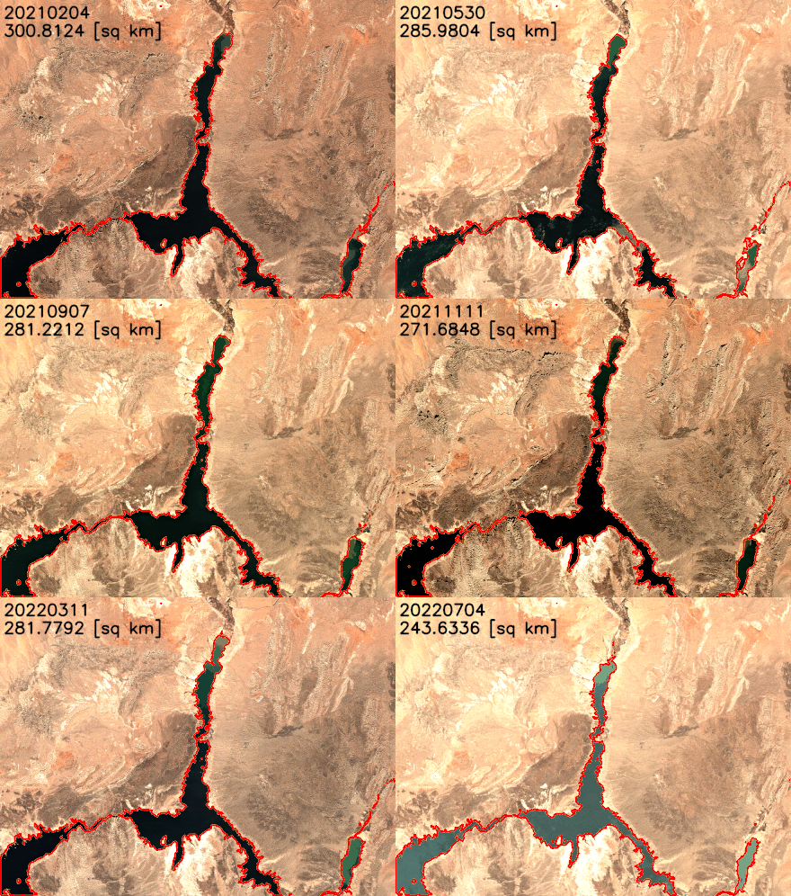
We plot the water surface area over time in the following figure. The water surface area clearly decreased between February 2021 and July 2022. In less than 2 years, Lake Mead’s surface area decreased from over 300 km2 to less than 250 km2, an 18% relative change.
We can also extract the lake’s boundaries and superimpose them over the satellite images to better visualize the changes in lake’s shoreline. As shown in the following animation, the north and southeast shoreline have shrunk over the last 2 years. In some months, the surface area has reduced by more than 20% year over year.

Conclusion
We have witnessed the impact of climate change on Lake Mead’s shrinking shoreline. SageMaker now supports geospatial machine learning (ML), making it easier for data scientists and ML engineers to build, train, and deploy models using geospatial data. In this post, we showed how to acquire data, perform analysis, and visualize the changes with SageMaker geospatial AI/ML services. You can find the code for this post in the amazon-sagemaker-examples GitHub repo. See the Amazon SageMaker geospatial capabilities to learn more.
References
[2] https://www.nps.gov/lake/learn/nature/overview-of-lake-mead.htm
[3] https://earthobservatory.nasa.gov/images/150111/lake-mead-keeps-dropping
About the Authors
Xiong Zhou is a Senior Applied Scientist at AWS. He leads the science team for Amazon SageMaker geospatial capabilities. His current area of research includes computer vision and efficient model training. In his spare time, he enjoys running, playing basketball and spending time with his family.
Anirudh Viswanathan is a Sr Product Manager, Technical – External Services with the SageMaker geospatial ML team. He holds a Masters in Robotics from Carnegie Mellon University, an MBA from the Wharton School of Business, and is named inventor on over 40 patents. He enjoys long-distance running, visiting art galleries and Broadway shows.
Trenton Lipscomb is a Principal Engineer and part of the team that added geospatial capabilities to SageMaker. He has been involved in human in the loop solutions, working on the services SageMaker Ground Truth, Augmented AI and Amazon Mechanical Turk.
Xingjian Shi is a Senior Applied Scientist and part of the team that added geospatial capabilities to SageMaker. He is also working on deep learning for Earth science and multimodal AutoML.
Li Erran Li is the applied science manager at humain-in-the-loop services, AWS AI, Amazon. His research interests are 3D deep learning, and vision and language representation learning. Previously he was a senior scientist at Alexa AI, the head of machine learning at Scale AI and the chief scientist at Pony.ai. Before that, he was with the perception team at Uber ATG and the machine learning platform team at Uber working on machine learning for autonomous driving, machine learning systems and strategic initiatives of AI. He started his career at Bell Labs and was adjunct professor at Columbia University. He co-taught tutorials at ICML’17 and ICCV’19, and co-organized several workshops at NeurIPS, ICML, CVPR, ICCV on machine learning for autonomous driving, 3D vision and robotics, machine learning systems and adversarial machine learning. He has a PhD in computer science at Cornell University. He is an ACM Fellow and IEEE Fellow.